Basic Model Loading and Usage

This example demonstrates how to load a BiosymModel and perform basic operations including forward kinematics, dynamics computations, and performance analysis.

We’ll use a simple pendulum model to illustrate the core functionality of the BiosymModel class.

import numpy as np
import jax.numpy as jnp
import matplotlib.pyplot as plt
import time
import timeit
import sys
import os


from biosym.model.model import load_model
from biosym.utils import states

Load the Model

First, we load a simple pendulum model from an XML file. The load_model function handles caching automatically, so subsequent loads will be faster. We toggle force_rebuild to True to ensure we load from the XML file directly and not from cache.

model_file = "tests/models/pendulum.xml"
print("Loading pendulum model...")
start_time = time.time()
model = load_model(model_file, force_rebuild=True)
load_time = time.time() - start_time

print(f"Model loaded in {load_time:.3f} seconds")
print(f"Model has {model.n_states} states and {model.n_constants} constants")

Loading pendulum model...
Replacing dynamic symbols in the EOM with the v_ states, this might take a while...
Lambdifying the EOM took 0.01990795135498047 seconds
Precompiling the Jacobian took 0.07780289649963379 seconds
Precompiling the confun took 0.07644414901733398 seconds
Precompiling the mass matrix took 0.06737685203552246 seconds
Precompiling the forcing took 0.08032512664794922 seconds
Model loaded in 0.947 seconds
Model has 8 states and 29 constants

Explore Model Structure

Let’s examine the structure of our loaded model to understand its components.

print("\n--- Model Structure ---")
print(f"Coordinates: {model.coordinates['names']}")
print(f"Speeds: {model.speeds['names']}")
print(f"Forces: {model.forces['names']}")

print(f"\nBodies in the model:")
for i, body in enumerate(model.dicts['bodies']):
    mass = body['mass'][0] if isinstance(body['mass'], list) else body['mass']
    com = body['com'] if 'com' in body else np.zeros(3)
    inertia = body['inertia'] if 'inertia' in body else np.zeros((3, 3))
    print(f"  {i}: {body['name']} (mass: {mass:.3f} kg, com: {com}, inertia: {inertia})")

print(f"\nJoints in the model:")
for i, joint in enumerate(model.dicts['joints']):
    print(f"  {i}: {joint['name']} (type: {joint['type']})")

--- Model Structure ---
Coordinates: ['q_hinge', 'q_hinge2']
Speeds: ['qd_hinge', 'qd_hinge2']
Forces: ['M_hinge', 'M_hinge2']

Bodies in the model:
  0: pole (mass: 1.000 kg, com: [0.0, 0.5, 0.0], inertia: [1.0, 1.0, 1.0, 0.0, 0.0, 0.0])
  1: pole2 (mass: 1.000 kg, com: [0.0, 0.5, 0.0], inertia: [1.0, 1.0, 1.0, 0.0, 0.0, 0.0])

Joints in the model:
  0: hinge (type: hinge)
  1: hinge2 (type: hinge)

Set Up Initial Conditions

Before running any computations, we need to set up the state and constant vectors. The model provides default values that we can use.

# Initialize state vector (positions, velocities, accelerations, forces, etc.)
states_dict = {
    "states": {
        "model": jnp.zeros(model.n_states),
        "gc_model": jnp.zeros(0),        # Ground contact model states
        "actuator_model": jnp.zeros(0),  # Actuator model states
    },
    "constants": {
        "model": jnp.array(model.default_values[model.n_states:]),
        "gc_model": jnp.zeros(0),
        "actuator_model": jnp.zeros(0),
    }
}

# Convert to proper dataclass format required by the model functions
states_obj = states.dict_to_dataclass(states_dict)

print(f"\nInitialized states vector with {len(states_obj.states.model)} elements")
print(f"Initialized constants vector with {len(states_obj.constants.model)} elements")

Initialized states vector with 8 elements
Initialized constants vector with 29 elements

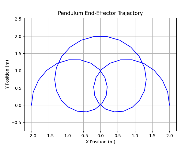
Forward Kinematics Analysis

Now let’s compute the forward kinematics for different pendulum angles to understand how the end-effector moves through space.

print("\n--- Forward Kinematics Analysis ---")

# Define a range of pendulum angles
angles = np.linspace(-np.pi/2, np.pi/2, 50)
angles2 = np.linspace(-2*np.pi, 2*np.pi, 50)
positions = []
velocities = []

# Set a small angular velocity for velocity computations
states_obj = states_obj.replace_vector("states","model",states_obj.states.model.at[1].set(0.5))  # angular velocity in rad/s

print("Computing forward kinematics for 50 different angles...")

for angle, angle2 in zip(angles, angles2):
    states_obj = states_obj.replace_vector("states","model",states_obj.states.model.at[0].set(angle))  # Set angle
    states_obj = states_obj.replace_vector("states","model",states_obj.states.model.at[1].set(angle2)) # Set angular velocity

    # Compute forward kinematics (positions)
    pos = model.run["FK_vis"](states_obj.states, states_obj.constants)[-1,:2]
    positions.append(pos.flatten())

    # Compute velocity kinematics
    vel = model.run["FK_dot"](states_obj.states, states_obj.constants)[-1,:2]
    velocities.append(vel.flatten())

positions = np.array(positions)
velocities = np.array(velocities)

print(f"Forward kinematics computed for {len(angles)} configurations")
print(f"Position output shape: {positions.shape}")

plt.plot(positions[:, 0], positions[:, 1], 'b-')
plt.title('Pendulum End-Effector Trajectory')
plt.xlabel('X Position (m)')
plt.ylabel('Y Position (m)')
plt.grid()
plt.axis('equal')
plt.show()

--- Forward Kinematics Analysis ---
Computing forward kinematics for 50 different angles...
Forward kinematics computed for 50 configurations
Position output shape: (50, 2)

Dynamics Computations

Let’s compute the equations of motion and examine the mass matrix and forcing terms for our pendulum model.

print("\n--- Dynamics Analysis ---")

# Set initial conditions: 45 degrees with some angular velocity
states_obj = states_obj.replace_vector("states","model",states_obj.states.model.at[0].set(np.pi/4))  # 45 degrees
states_obj = states_obj.replace_vector("states","model",states_obj.states.model.at[1].set(1.0))         # 1 rad/s angular velocity

# Compute equations of motion residual
eom_residual = model.run["confun"](states_obj.states, states_obj.constants)
print(f"EOM residual: {eom_residual}")

# Compute mass matrix
mass_matrix = model.run["mass_matrix"](states_obj.states, states_obj.constants)
print(f"Mass matrix shape: {mass_matrix.shape}")
print(f"Mass matrix:\n{mass_matrix}")

# Compute forcing terms (Coriolis, centrifugal, gravity)
forcing = model.run["forcing"](states_obj.states, states_obj.constants)
print(f"Forcing terms: {forcing}")

# Compute Jacobian for sensitivity analysis
jacobian = model.run["jacobian"](states_obj.states, states_obj.constants)
print(f"Jacobian shape: {jacobian}")

###############################################################################

--- Dynamics Analysis ---
EOM residual: [[15.19756178]
 [ 4.7924855 ]]
Mass matrix shape: (2, 2)
Mass matrix:
[[4.04030231 1.52015115]
 [1.52015115 1.25      ]]
Forcing terms: [[15.19756178]
 [ 4.7924855 ]]
Jacobian shape: States(model=(2, 1, 8), gc_model=(2, 1, 0), actuator_model=(2, 1, 0), h=None)